Dickimaw Books Blog 
From JpgfDraw to FlowframTk: A Vector Graphics Application Inspired by Acorn’s !Draw 🔗

\special) on an Archimedes. These images were vector graphics (shapes defined by a set of control points) and were created with Acorn’s !Draw application. When I began to migrate over to Linux in the late 1990s to early 2000s, the one thing I really missed was Draw.
Nowadays, there are notable vector graphics applications available, but, back then, they either didn’t exist or existed only in an early stage or they existed but I didn’t find them (it’s much easier to search for things now) or they didn’t run on Linux. The ones I tried didn’t have the features that I particularly wanted and knew how to easily achieve in Draw, which was quite frustrating.
The types of images that I wanted to create roughly fell into two categories: diagrams to incorporate into a LaTeX document for articles or reports, and flyers or posters to advertise events for organisations I belonged to. Depending on the complexity of the image, I would either use pstricks (the drawing code is written in the LaTeX document source using the environment and commands provided by that package) or I would switch back to RISC OS and use Draw (a Windows, Icons, Menus and Pointers, WIMP, application). Since I couldn’t include the DrawFile with \special once I was back on Linux, I had to convert the image to EPS from Draw running on a RiscPC and transfer it across via a floppy disk to my Linux laptop.
There were a number of focal points: the frustration in having to switch on another computer (albeit one with an operating system that starts up and shuts down quickly), newer laptops not having a floppy drive, a growing desire to move away from the old LaTeX+dvips+ps2pdf compile build to using the newer pdfLaTeX, the arrival of the pgf (portable graphics format) package by Till Tantau, and a decision to move away from C to Java. Not being able to find a suitable replacement that was already available, it was time to write one that had the features that I wanted: an interface similar to Draw with the ability to export to a format suitable for use with pdfLaTeX.
I’d had some experience writing WIMP applications on RISC OS, which used a polling loop and finite state machine, and I’d also written a graphical user interface (GUI) application that ran on Windows NT for work. (I have no recollection of how I wrote it, other than that it was in C, but I had to use a commercial library that was only available on Windows so I didn’t have much choice.¹) Java’s Abstract Window Toolkit (AWT) and the Swing library built on AWT are event driven, which is much easier to code. The other great thing about Java is that it’s platform-independent. So I can write the application on Linux and people can use it on any operating system that has the Java Virtual Machine (JVM) installed on it. Whereas with compiled languages, such as C, the application will only run on the operating system it was compiled on. Cross-platform support requires a team of developers with access to multiple different platforms or virtual machines and with knowledge of the little quirks and idiosyncrasies of the target platforms. Java is a useful language for a solo developer, particularly a hobbyist working for free.
So I wrote a vector graphics application in Java that could create PGF drawing code suitable for inclusion in a LaTeX document. And since I’ve never been good at naming things, I called it JpgfDraw. Unfortunately I lost early versions due to a hard disk failure. The earliest reference in my CHANGES file is for version 0.1.4b and the earliest bug report that I can find was sent in 2006 for version 0.1.8b. The CTAN new package announcement wasn’t until August 2008 so I must have had it available for testing (on “theoval”) for at least a couple of years before I uploaded it.
I incorporated most of the main features that Draw had, but not the interpolation or grading functions. Whilst I admittedly had a lot of fun playing around with them when I regularly used RISC OS, I didn’t actually need them or have the time to work out the maths to implement them. Maybe I’ll get round to it one day.
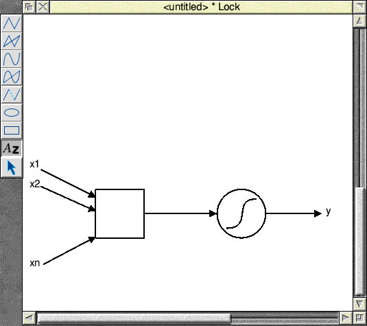
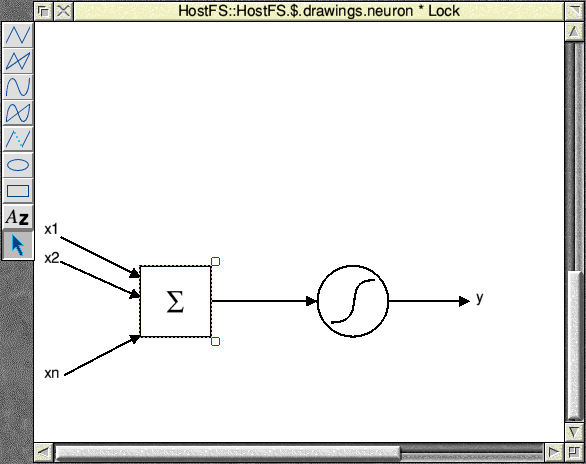
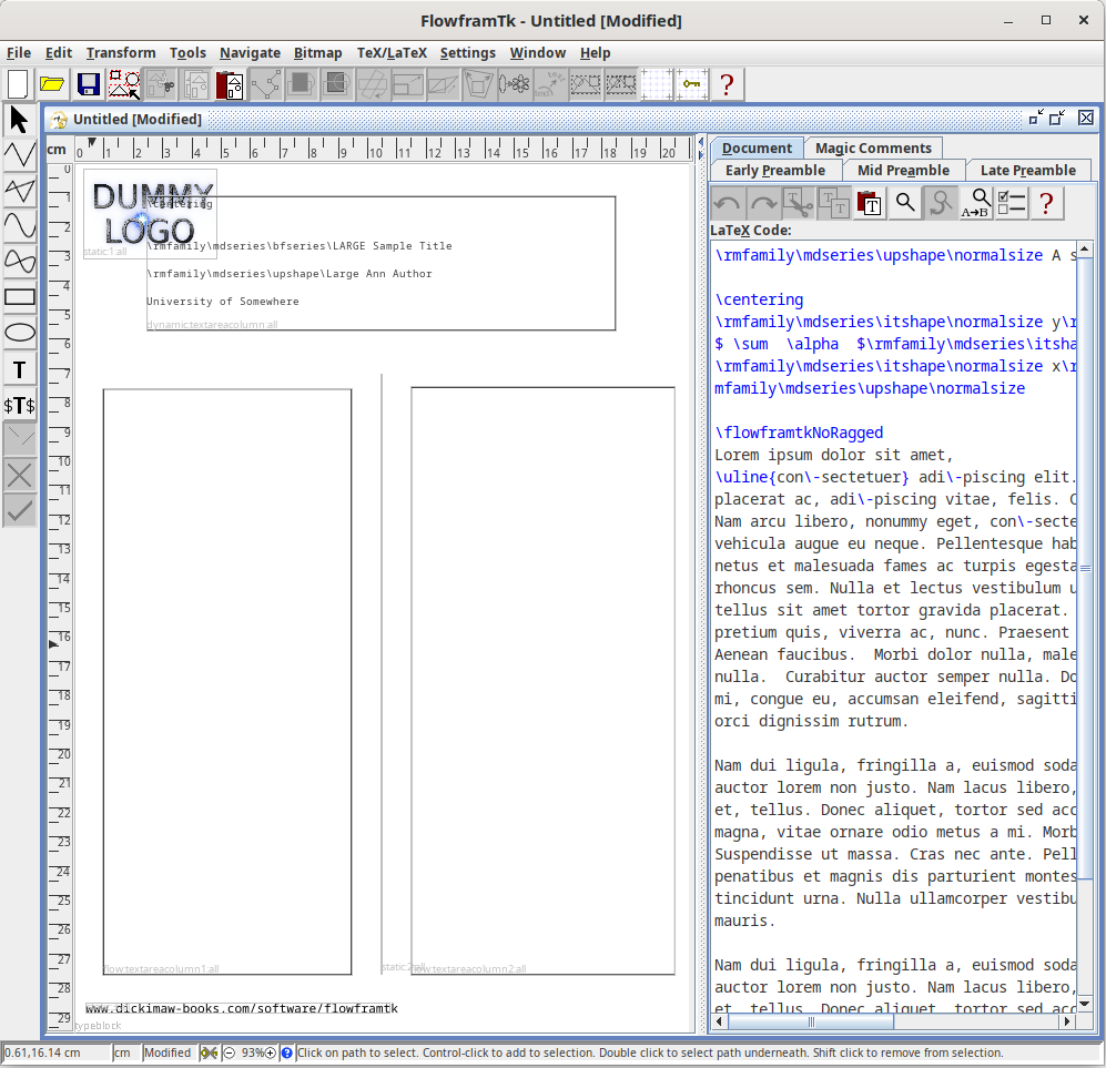
Below shows a screenshot of Draw (running in RPCemu) with an image of an artificial neuron. (A simplified version of an image from my PhD thesis.) This consists of a square created with the rectangle tool, a circle created with the ellipse tool and lines with triangle arrow heads. The annotations were created with the text tool.
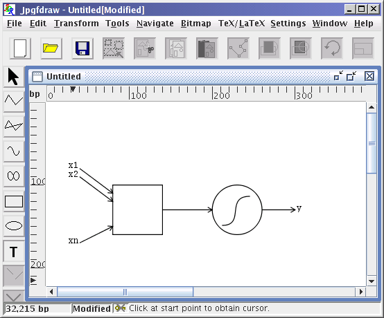
The image next to that is a screenshot from JpgfDraw (from version 0.5.6b or earlier) showing a similar diagram. The arrow heads and font are a little different but otherwise the pictures are essentially the same kind of construct.
Both applications have a similar toolbox on the left but the tools are in a different order. In Draw, they are: open line mode, closed line mode, open curve mode, closed curve mode, move to (for use during path construction), ellipse mode, rectangle mode, text mode and select mode. In JpgfDraw, the select tool comes first, followed by the path construction modes: open line, closed line, open curve, closed curve, rectangle, ellipse, and then the text mode. After that are the buttons that are only available when a new path is under construction: move to, cancel, and finish. All shapes are paths made up of moves, lines or cubic Bézier curves, with the option to open or close the path. For both applications, the rectangle and ellipse modes are a convenient shortcut that create a shape with control points that can then be edited as general paths.
One thing that a Draw user might find confusing is that I changed the terminology for the text created with the text tool. In Draw, each line of text is called a “text line”. For some reason or other, I called the analogous object in JpgfDraw a “text area”, which is something completely different in Draw but I’ll return to Draw’s “text area” later.
Since I specifically designed JpgfDraw with the aim of export to LaTeX code, each text area has both canvas attributes (the text and the font used to render it on the screen) and LaTeX attributes (the code to use when exporting to a LaTeX file). Below shows the first of the text areas in the above drawing in the edit dialog.
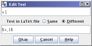
The top field is the canvas text (“x1”). The second field is the text that should be written to the LaTeX file ($x_1$).
The “Same” and “Different” radio buttons disable or enable the second field. The font settings also have both a canvas and a LaTeX attribute.
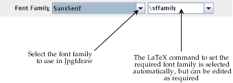
The font family has the font name for rendering on the canvas (for example, the generic “SansSerif” name or a specific font family such as “Liberation Serif”) and the most appropriate LaTeX font family declaration (for example, \sffamily or \rmfamily). Similarly for the weight, shape and size. Depending on your application settings, the font size declaration may either be a relative declaration (such as \large) or an explicit size. The font declarations are set automatically based on the image font settings, but you can change them if they’re not appropriate. The relative size selection will need the size of the normal font. This is also needed for other features and should ideally be set up for the image when it’s new.
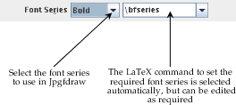
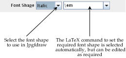
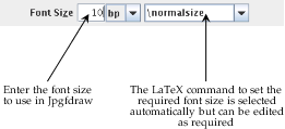
When setting a size, the unit is as for TeX: pt (a TeX point), bp (a “big point”, that is a PostScript point), in (inch), cm (centimetre), mm (millimetre), pc (pica), dd (didot) or cc (cicero).
Below is a modification to the above image of an artificial neuron. In Draw, I’ve added a text line with a summation sign by switching to the Sidney font and selecting the appropriate character (0xE5) from the !Chars application. In JpgfDraw, I’ve added the Unicode n-ary summation sign (∑ U+2211) using the Insert Symbol dialog box that can be obtained through JpgfDraw’s text area popup menu. In both cases, I switched to text mode and inserted the cursor inside the square that I’d created with the rectangle tool. I then grouped both the ∑ text and the square and used the horizontal and vertical justify functions to centre the text within the rectangle.
In both cases, the screenshot shows the group still selected. In Draw, this is shown by a dotted rectangle with two “ears”: little squares at the top right and bottom right corner. These can be used to rotate or scale the selected object. In JpgfDraw, the selection is shown by a dashed rectangle. It doesn’t have any ears showing, but it does have six hotspots that can be enabled. They’re not set by default as they can be easily hit by accident on small bounding boxes. If you want them, you can switch on the setting.
Again, in JpgfDraw I’ve used the edit text dialog to set the alternative text to use when the image is exported to a LaTeX file. The problem here is that the font used in the LaTeX document is likely to be different to the one used to render the text on the canvas. This means that the large sigma summation symbol may be wider or narrower or shorter or taller in the document compared to the way it’s shown on the canvas, which would cause it to be off-centre in the document if the text node is positioned at the bottom left corner of the text area’s bounding box.
The text area attributes in JpgfDraw additionally include anchor settings which don’t affect the way the text is drawn on the canvas but do change the point where the text is positioned in the exported file. The justification function automatically changes the applicable anchor setting but you can change it yourself, for example, if you are manually aligning some text rather than using the justify sub-menu.
The exported LaTeX file contains PGF picture code encapsulated in the pgfpicture environment. I still have a printout of the User’s Guide to the PGF Package, Version 0.65 (November 4, 2004) that I used as a reference when I was first designing JpgfDraw. It’s 26 pages long. There was no TikZ and no libraries. Path construction was implemented with commands like \pgfmoveto and \pgflineto. There were eleven line markers: \pgfarrowlargepointed{size}, \pgfarrowtriangle{size}, \pgfarrowcircle{size}, \pgfarrowdiamond, \pgfarrowdot, \pgfarrowpointed, \pgfarrowround, \pgfarrowsquare, \pgfarrowbar, \pgfarrowsingle, and \pgfarrowto, which could be combined or reversed. So the early versions of JpgfDraw implemented these markers and used the corresponding command when exporting the image. Only the first three had a size argument, so they were the only ones that had a configurable size within JpgfDraw.
As PGF developed and provided more sophisticated ways of defining markers, I decided to stop trying to keep up and instead made the export function write the PGF code to draw each marker as a path. The output isn’t particularly readable, but I never had any reason to edit the files exported by JpgfDraw. My aim was for JpgfDraw to be sufficiently configurable to not need to, and the less parsing and calculating that has to be done within LaTeX, the faster the overall document build time. The original eleven markers are still present. If you encounter any markers within JpgfDraw (and latterly FlowframTk) that don't have a configurable marker size, then they are the legacy markers corresponding to those PGF arrow commands that didn’t have a size argument. There are now newer markers that can be used instead. Path construction commands have also changed. Later versions of JpgfDraw switched from \pgflineto to \pgfpathlineto etc.
By way of comparison, at the time of writing this I have pgf version 3.1.11a installed and the manual is 1323 pages long. The PGF bundle has grown onwards and upwards to a fantastic flexible drawing system. These days, if I need to write drawing code within a LaTeX document then I will use TikZ, but FlowframTk still uses the pgfpicture commands that are now in PGF’s basic layer.
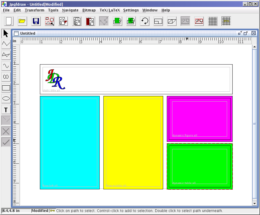
When text areas are exported, the text is placed in the mandatory argument of \pgftext, with the position and the horizontal and vertical alignment determined according to JpgfDraw’s anchor setting. Raster (bitmap) images can also be included. Acorn’s Draw also supports the inclusion of Sprites (Acorn’s raster format) or JPEG files and the DrawFile format has the raster data embedded. Since JpgfDraw was specifically designed for export to LaTeX, the raster data must be in a form that can be input using either \pgfimage or \includegraphics, so JpgfDraw simply stores the bitmap file path (to fetch the data to render it on the canvas) and the LaTeX path to use in the exported file (as well as a transformation matrix). This means that if you change the location of the linked bitmap file you will need to update the information in JpgfDraw. The image below shows JpgfDraw with a bitmap image, a path and a text area.
This dealt with my first goal of wanting a graphical interface to create image files that I could simply insert with \input into a LaTeX document. My second goal was to be able to design a complete document, such as a poster or flyer. I could just use the File > Print menu item and print the image directly using the image’s page size. This would print the image just as it’s rendered on the canvas. But what if I want the text to be properly typeset? So I added a second export function that creates a complete LaTeX document with an empty header and footer and just the image in the document environment. It’s already necessary to identify the normal font size in order for the correct relative size declarations to be selected. The normal font size can be one of: 8, 9, 10, 11, 12, 14, 17, 20, and 25. This setting determines both the document class option and the document class: article for 10, 11 or 12, a0poster for 25, and extarticle for the others. The geometry package is used to set up the page size.
Remember that each of JpgfDraw’s text areas is exported in the argument of \pgftext. This restricts the content. You could set the alternative LaTeX text to a paragraph encapsulated within a \parbox command or minipage environment, but it then becomes hard to gauge the extent when viewing it on the canvas.
While I was working on JpgfDraw, I was also working on the flowfram package, which I first uploaded to CTAN in July 2005. Again, I was trying to find a way to create a poster, but this time not a graphics-filled flyer. This type of document was for academic poster presentations at conferences. It needed to be big (A0), with columns of text, likely including mathematical content, and a logo and affiliation in one corner, and maybe a prominent figure or table.
The LaTeX kernel provides one column and two column modes. The multicol package provides a way of setting up multiple columns, but it wasn’t sufficient for this type of layout. What I needed was to be able to extend the way that the output routine deals with two column mode to allow for an arbitrary number of columns with arbitrary dimensions and positions. This requires hacking the LaTeX internals which is risky and prone to conflict with other packages. It can also come apart if the LaTeX kernel changes, which it has done quite significantly over the past decade. I released flowfram 2.0 (2025-11-24) late last year with a major rewrite to allow for the changes, but it still needs to do some tampering to achieve the desired effects.
Way back, in olden days of yore, CTAN had an eight dot three filename restriction. I wanted to call the package “flowframe”, but the final “e” had to be sacrificed to satisfy this requirement. The filename restriction has thankfully long since been lifted, but the package name remains flowfram. If I talk or write about “flowframe data”, I mean settings relating to the flowfram package, although the package actually provides three types of frame: flow, static and dynamic.
A flow frame is essentially like one of LaTeX’s columns used in two column mode but it has an associated position, width and height. It also has a page list (and, later, an exclusion list) identifying which page or pages that it’s valid on. The page list can be “all” (all pages), “none” (no pages), “odd” (odd pages only), “even” (even pages only) or a comma-separated list of individual pages or page ranges. These have to be plain numbers, such as 1 or 2, not formatted numbers (i or ii) because the flowfram code added to the output routine needs to be able to make numerical comparisons. The page ranges may either be closed (for example, 2-8) or open (for example, <4 or >12). Originally, flowfram just used the page counter but this causes complications when it’s reset (for example, by \mainmatter) so there’s now an absolute page setting to allow the absolute page number to be referenced in the page lists instead. You can change the page list mid-document (which is why there’s a “none” setting) but you need to be careful where to place it in relation to when the output routine needs to query it.
In LaTeX’s normal two column mode, the document text starts filling up the first column. Once it’s full, the output routine saves the content (in a box) and switches to the second column. Once that has filled, both columns are placed on the page and the page is shipped. The page counter is incremented and the output routine switches back to the first column. This is a bit of a simplification (there’s also the floats, footnotes etc to take into account), but the same kind of process happens with the flow frames. The first flow frame (in the order in which they were defined) that is valid on the current page is selected and the document text starts filling up as usual. When the column is full, the content is saved in a box associated with that flow frame and the output routine selects the next flow frame that’s valid on the current page. If there are none left, flowfram’s special laying-everything-out-on-the-page function is used before shipping out the page. The page counter is incremented as usual, and the output routine will search for the first flow frame to be defined on this new page. If none are defined, an empty page is shipped. Although it might not actually be blank, because there are two other types of frame that may place content on the page.
A static frame also has a position and a width and height. It shares other attributes with flow frames, such as an associated page list, but the content must be explicitly set using either an environment or a command. The content is placed inside a minipage with the frame’s dimensions and it’s saved in a box. This means that the content is typeset as soon as it’s assigned to a static frame. So if the content includes a command that has changing output (such as \thepage), the content is fixed in place with the value that command had when the static frame content was set. The static frame’s content won’t change until it’s explicitly set to something else. (Unless you switch on the clear attribute, which automatically clears the content when a page is shipped out.)
A dynamic frame also has a position and a width and height and it shares many of the static frame attributes and also has its content placed inside a minipage environment (previously a \parbox) but, in this case, when the dynamic frame content is set, it’s stored in a token list variable. This means that it’s not typeset until the special laying-everything-out-on-the-page function puts it on the page, using whatever is the current definition or value of any commands or counters contained within it. Dynamic frames also have a style setting, which isn’t available for static or flow frames. The value is the control sequence name of a formatting command (such as bfseries) or a text-block command that has a single argument (such as textbf). Note that there’s no leading backslash. This is used to format the content of the dynamic frame. If you need multiple styles (for example, bold and italic), you will have to define a wrapper command to use. Alternatively, you can just place the required formatting commands at the start of the content, as you would have to do for static frames.
Again I’m going to simplify things, but content is typically placed on a page as follows. Start at the top left corner of the page and move right by 1 inch plus either \oddsidemargin or \evensidemargin, and down by 1 inch plus \topmargin plus \headheight. This is the point where the bottom left of the page header goes. Then move down by \headsep plus \textheight. This is where the bottom left of the first column in two-column mode or the column in one-column mode is placed. From flowfram’s point of view, this is the position or origin of the typeblock. After that, move down by \footskip and you’re at the position where the page footer goes.
The page layout should be established before flowfram is loaded. For example, if you want to load the geometry package, it’s best to do this and set up the layout before flowfram is loaded. As from version 2.0, flowfram has a hook in case geometry is loaded afterwards, but any subsequent changes with commands like \geometry or explicitly changing any of the page layout lengths is likely to confuse flowfram. This new version of flowfram also introduces two new lengths: \typeblockwidth and \typeblockheight, which identify the width and height of the typeblock. These are initialised to \textwidth and \textheight. All flow frames should lie within this region. Static and dynamic frames may be outside of the typeblock.
The position attribute for all types of frame indicates the bottom left corner of the frame and is relative to the typeblock origin, where a positive x value indicates to the right of the origin and a positive y value indicates above the origin. Negative x and y values shift left and downwards, respectively. Each frame has two positions: the odd page position and the even page position. Remember that these are both relative to the typeblock origin which may shift on even pages if \oddsidemargin and \evensidemargin are different. For a one-sided document, only the odd page position and \oddsidemargin is used. Flow frames typically have the same position for odd and even pages, just relying on the difference between \oddsidemargin and \evensidemargin to shift them, but static and dynamic frames may have different positions on even pages. For example, they might be placed on the right of an odd page and on the left of an even page.
The header and footer code is removed from its usual place and put in the laying-everything-out-on-the-page function. This is because the flowfram package has a feature that transfers the header and footer into dynamic frames. (Make sure to have v2.0+ installed to ensure that the tagging code is retained.) These special dynamic frames should not have their content changed or cleared. Instead, use the custom page styles and settings provided by flowfram. The position (odd or even), size, font style and other dynamic frame attributes can be changed in the usual way.
The laying-everything-out-on-the-page function works as follows:
- All static frames that are valid on the current page are placed in their position relative to the typeblock origin (according to the current odd/even setting) in the order in which they were defined.
- If the header hasn’t been moved into a dynamic frame, it’s placed in its usual position above the typeblock.
- If the footer hasn’t been moved into a dynamic frame, it’s placed in its usual position below the typeblock.
- All flow frames that are valid on the current page are placed in their position relative to the typeblock origin (according to the current odd/even setting) in the order in which they were defined.
- All dynamic frames that are valid on the current page are placed in their position relative to the typeblock origin (according to the current odd/even setting) in the order in which they were defined.
There’s no interaction between the frames. The text in one frame doesn’t budge out of the way of another frame. Any frame higher up the stacking order that has an overlapping position will be drawn on top. Static frames can therefore be used for background effects.
For example:
\newflowframe{3in}{6in}{0pt}{0pt}
\newdynamicframe{5in}{1in}{0pt}{7in}
\newflowframe{3in}{6in}{3.5in}{0pt}
\newstaticframe{8in}{7in}{-1in}{-1in}
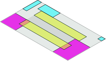
The above code defines two flow frames both with width 3in and height 6in, a dynamic frame higher up the page and a static frame positioned below and to the left but overlapping the other frames. The document text will start in the first flow frame (on the left) and continue in the second flow frame (on the right). If the flow frame definitions were swapped round, the text would start on the right and continue on the left.
Despite the fact that the static frame was defined last, it will be drawn first. The two flow frames are drawn next, and finally the dynamic frame is drawn.
It’s a bit fiddly working out all the dimensions of the page layout and frame positions and sizes.
If only there was a graphical application to help.

In JpgfDraw, you can assign flowframe data to an object and export the information as a LaTeX class or package that loads both geometry and flowfram, but first you must establish the typeblock because JpgfDraw needs to know where the typeblock origin is in order to calculate the relative positions from it, and also it will need the information to set up the page geometry.
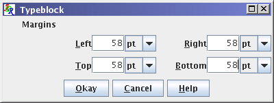
Once the typeblock has been set, a grey rectangle is drawn on the canvas showing its location. You can then select an object and assign flowframe data to it.
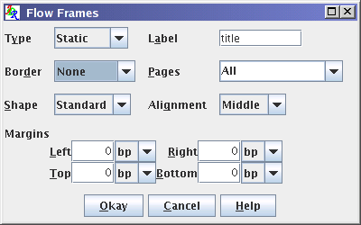
The object’s bounding box is used to establish the position and size of the frame. The object itself won’t be exported (to a class or package file) unless the border option is set. If it is set, the object will form the frame’s border and background. This is true even if the selected object is a text area. The text in the text area will be considered a background effect and not the frame content. Any object that doesn’t have flowframe data assigned to it won’t contribute to the export. This means that you can create objects that are simply guides to help position the objects with flowframe data.
Once you have exported the flowframe data to a class or package, you can load it in the usual way in a LaTeX document with \documentclass or \usepackage.
So the JpgfDraw export options include:
- Create a file containing a
pgfpictureenvironment that replicates the image as closely as possible, allowing for LaTeX fonts and alternative text, that can be input into a document. - Create a file containing a complete self-contained LaTeX document that replicates the image as closely as possible, allowing for LaTeX fonts and alternative text, that can be compiled/built/typeset by LaTeX.
- Create a cls or sty file containing a class or package that loads flowfram and defines the page layout that can be used by a LaTeX document. The canvas objects aren’t rendered in the document unless they’re set as frame borders.
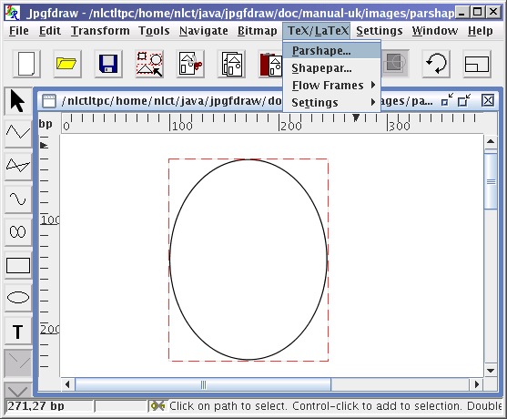
I straddle the sciences and the arts. I have a degree in mathematics and a PhD in electronic systems engineering, but I also have a diploma in creative writing. My main interest in writing is prose fiction, but I have also written some poetry. For one of the poetry assignments, I wrote a poem called “The Dripping Tap” which, in of itself, isn’t particularly interesting, but I styled each verse in the shape of a droplet, offset at intervals down the page. The poem didn’t exactly knock the socks off my fellow students, but they were impressed by the shaped paragraphs which, naturally, I had typeset in LaTeX but I had designed the paragraph shape in JpgfDraw.
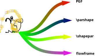
TeX itself has a primitive called \parshape that can shape a paragraph according to a set of indents and line widths. It’s limited as to the type of shapes it can produce. The shapepar package provides a more flexible method with \shapepar. In both cases, the syntax requires some calculation, even more so for \shapepar. So I added a feature to JpgfDraw where you can select a path (not a text area or bitmap) and JpgfDraw will calculate the required parameters. It will then display a file chooser and the applicable command (\parshape or \shapepar) and its parameters will be saved in that file. The file can then simply be \input at the start of the required paragraph. This is the only TeX feature of JpgfDraw that’s not specific to LaTeX as \parshape is a primitive and shapepar is a generic package so it can be used with Plain TeX as well.
The function works by creating horizontal scan lines that pass through the shape at vertical intervals given by the baseline skip value. This means that you need to remember to set the normal font size first to match that used in your document. Each of the predefined set of normal font sizes is associated with the appropriate \baselineskip value. The shapepar package later introduced \Shapepar which has the same syntax as \shapepar. You can choose which command to write to the file. (Even more recently, \cutout has been added to shapepar but that’s not supported by JpgfDraw.)
\parshape
If you want a shaped paragraph in a flow frame, you can use this method. However, if you want the content of a static or dynamic frame shaped you can instead use the shape attribute but only do this if the frame content is just normal-sized text.
It was brought to my attention that the first three letters of JpgfDraw are “jpg” which caused some confusion over the purpose of the application, suggesting that it might have something to do with JPEG files. I decided that perhaps it would be best to rename the application to avoid confusion. Since there were a number of other (La)TeX-aware vector graphics applications, I decided the new name should focus on the one unique (as far as I know) aspect of the application, and that’s its ability to create flowfram code. The last version of JpgfDraw was 0.5.7b and then I renamed it FlowframTk in 2019. The version numbers follow on, so the first version of FlowframTk was 0.6. The “jdr” abbreviation (from JpgfDraw) used for the .jdr file format extension and in various other places has been retained (such as in JDRView, a simple viewer provided with JpgfDraw and now bundled with FlowframTK). I also changed the logo, adapting the Dickimaw parrot logo with one of the paths showing in edit mode.
It’s now possible to set the contents of a static or dynamic frame from within FlowframTk as well as code that should be added to the preamble, package or class, depending on whether or not the export is to a complete LaTeX document, package or class. In the case of export to package or class, \usepackage will automatically be replaced with \RequirePackage.
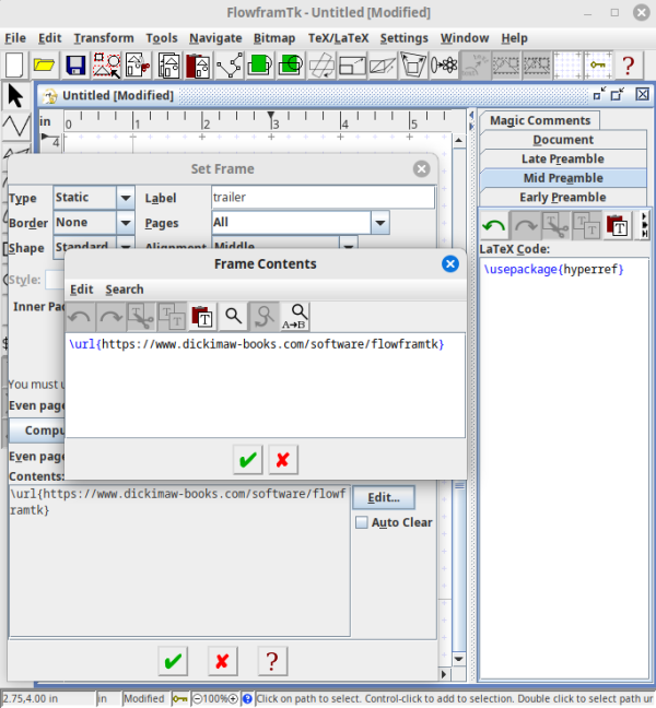
There are two types of export to complete LaTeX document. The first has already been mentioned above. The document body simply contains the PGF drawing code to replicate the image. The second is a document that loads the flowfram package, sets up the frames and the document content can either be provided in FlowframTk or the content can simply generate blank pages in order to view the layout before adding the actual text.
There are also two export to PDF functions, which use the applicable export to complete LaTeX document to create a .tex file in a temporary directory and then pdflatex is automatically run. The PDF is then moved to your chosen location and the temporary directory and its contents are removed. You can replace pdflatex with another application, such as latexmk or arara. In the latter case, you will need to add the special arara comment directives, which can be done in the “Magic Comments” panel. This means that the entire content of a document as well as the frame definitions can be bundled up in the jdr file. (I don’t recommend this for a large document as the code editor provided with FlowframTk is fairly basic and doesn’t include a spell-checker.) You will, obviously, need to have a TeX distribution installed.
Many new features have been added over the years, such as text-paths, symmetric shapes, patterns, improved interface, and automatically setting the alternative LaTeX text with character to command mappings. There are screenshots available that demonstrate some of these features but, after over twenty years, I’ve finally added support for importing Acorn DrawFiles and this brings me back to Draw’s “text area”, which really is an area (not a line) of text.
Acorn designed Draw not only as a vector graphics application but also as a desktop publishing (DTP) application. It’s possible to define columns and have text flow from one column to the next (sound familiar?) When FlowframTk imports a DrawFile that has a Draw text area, FlowframTk will create a rectangle for each column and assign flowframe data.
A DrawFile text area can be created by dragging and dropping a plain text file onto Draw. If the text doesn’t start with special markup then just one column is created but greater control can be had by starting the text file with text area markup. The Archimedes user guide provides an example:
\! 1
\AD
\D2
\F0 Trinity.Medium 24
\L24
\P24
\0A sample text area...
where
\! 1 identifies the content as a text area, \AD indicates full justification, \D2 indicates two columns, \F0 sets font 0, \L24 and \P24 set the line and paragraph spacing, respectively, to 24 points, and \0 selects font 0. This is then followed by the content of the text area.
When FlowframTk imports a DrawFile with a text area, it will ignore line and paragraph spacing instructions since LaTeX will deal with that. You can use the preamble areas to, for example, load setspace if you need to adjust the line spacing or to load a font package, such as lmodern. FlowframTk recognises some common font names and will try to provide appropriate declarations, such as \rmfamily, but more important is the character encoding as the characters need to be mapped to the most appropriate Unicode character. If the font name is unrecognised, FlowframTk will assume it has the same encoding as Trinity, which is similar to Latin-1.
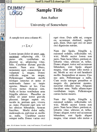
Multi-column text areas will be converted to flow frames and the content will be added to the document body panel. Single-column text areas will be converted to dynamic frames with the content set. The image below shows Draw with a single-column text area spanning the top with a title, author and affiliation and a two-column text area below with sample text. The main font is Trinity but it’s necessary to switch to Sidney for the mathematical symbols (summation and alpha). When FlowframTk imports a DrawFile, if it encounters Sidney in a text area it will automatically insert the maths-shift $ symbols on either side and apply the maths-mode mappings (after the conversion from Sidney encoding to Unicode). There is also a vertical line between the two columns of the lower text area, an embedded JPEG with a sample logo at the top right, and a text line along the bottom with a URL.
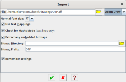
Since I’m using an emulator, the actual DrawFile is stored on Linux using the NFS style suffix (a comma followed by a three-digit hexadecimal) to identify the file type. This means that when I import the DrawFile in FlowframTk running on Linux, the DrawFile file, which is simply called DTP on RISC OS, actually has the filename DTP,aff.
I've used quite a large font in the DrawFile, so in the import dialog, I’ve set the normal size font to 17. I can also choose whether or not to extract the JPEG file. (There’s currently no support for imported Sprite files.) The filename for the extracted image will be constructed from the given prefix followed by a number that’s incremented for each extracted image. If you don’t specify a destination directory, the imported bitmaps will be saved in the current working directory.
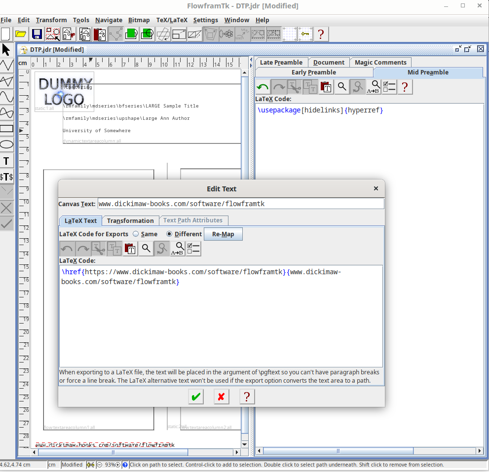
The single column with the title in the DrawFile is imported into FlowframTk as a rectangle with flowframe data assigned with the type set to dynamic and the content set to the code obtain from parsing the column text. The two-column area is imported as two rectangles both with flowframe data assigned with the type set to flow. Their content is put into the document code tab, but the markup and the character coding has to be converted. If any Draw text areas are detected, all other objects imported from the image will be set as static frames with the border set. In this example, that means the vertical line between the two columns, the extracted JPEG, and the text line with the URL. I can edit the text to use \href or \url in the alternative LaTeX text. (The Edit Text dialog has changed since the early days of JpgfDraw. There’s now more room for the LaTeX alternative code.) Remember to add hyperref to the mid or late preamble code.
This DTP example is rather more complicated than the example given in the Acorn User Guide. The centred line of maths is created by switching the paragraph justification (\AC), then switching to an italic font for the y, switching to an upright font for the equal sign, then to the Sidney font for the summation and alpha, then to a small italic font for the subscript but the baseline needs to be lowered (\V-9) before the i and raised back up again (\V9) afterwards and so on until the end of the formula. The justification is then reset back to full (\AD).
Reverting back to full justification is a bit awkward as LaTeX doesn’t provide a command analogous to \raggedright, \raggedleft and \centering so FlowframTk will use \flowframtkNoRagged, which is provided by flowframtkutils v2.2+. It’s likely that you will need to do some editing after importing, so you may prefer to remove \flowframtkNoRagged and add grouping to localise any changes.
In this case, the entire paragraph with the formula will need editing as there’s no way for FlowframTk to detect that it should be in displayed math-mode. The imported code that’s placed in the document environment is unnecessarily complicated and omits the vertical shifts, but has picked up the soft hyphen (\- which has the same markup for both the Draw text area and TeX):
\rmfamily\mdseries\upshape\normalsize A sample text area column \#1.

\centering
\rmfamily\mdseries\itshape\normalsize y\rmfamily\mdseries\upshape\normalsize  = $ \sum  \alpha  $\rmfamily\mdseries\itshape\scriptsize i \rmfamily\mdseries\itshape\normalsize x\rmfamily\mdseries\itshape\scriptsize i\rmfamily\mdseries\upshape\normalsize

\flowframtkNoRagged
Lorem ipsum dolor sit amet,
\uline{con\-sectetuer} adi\-piscing elit. […]
Once the formula has been edited, there’s no need for any of the declarations. Tidied up, the document environment now begins:
A sample text area column \#1.

\[
 y = \sum \alpha_i x^i
\]

Lorem ipsum dolor sit amet,
\uline{con\-sectetuer} adi\-piscing elit.
Note that the underlining markup (\U) was detected, but there’s only limited support and no support for nested underlining. The underlined content is encapsulated with \uline and \usepackage[normalem]{ulem} was automatically added to the early preamble tab. This may need editing if a different command or package is preferred.
In addition to the early, mid and late preamble code that’s saved in the JDR file, it’s also possible to set up a default preamble block that will always be inserted at the start if you export to a complete LaTeX document. I have my default preamble block set to:
\usepackage{iftex}
\ifpdftex
 \usepackage[T1]{fontenc}
 \usepackage{lmodern}
\else
 \usepackage{fontspec}
\fi
Since the columns are narrow, I’ve also added microtype to the early preamble code:
\usepackage{microtype}
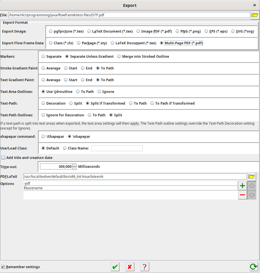
I can now export to a complete document that uses the flowfram package to layout the page, but here I’ve decided to use the export to a PDF document. The export setting is actually labelled “Multi-Page PDF” because it has the potential to have multiple pages. This is in contrast to the “Image PDF” setting, which will always be a single-paged PDF that simply displays the image.
The Export dialog is quite complicated, but most of the options aren’t applicable here and can be left in their default states. In this case, I’ve switched the default pdflatex call to latexmk, although that’s not necessary with this simple example as there are no cross-references. (If you prefer to use arara, you can place the arara directives in the Magic Comments tab. Likewise for any other build tool that relies on special comments.)
The document text is actually too long for one page. Draw simply truncates the text to fit within the designated columns, but the full text is still saved in the DrawFile and FlowframTk adds it all to the document environment. This means that the resulting PDF actually has two pages. The different font and paragraph settings (indent and skip) also make a difference in how much text can fit into each column.
The latest version can be found in the Releases area of FlowframTk’s GitHub repository. In the Assets area, there should be a link to the installer. For example, flowframtk-0.9.1-installer.jar for version 0.9.1 (the latest version at the time of writing). You will need to have Java installed. Depending on your system, you may be able to just double-click on the installer file. Alternatively, you can run it from the command line. For example:
java -jar flowframtk-0.9.1-installer.jar(Replace
0.9.1 as applicable.)
I intend to upload FlowframTk to CTAN after I have done some more testing. (After over two decades, it may even have reached version 1.0 by then!)
¹The one thing I do remember is that a TV crew visiting the institute where I worked filmed me with the application running while I talked about food-borne botulism and tried to explain that risk isn’t a number as it’s a concept that encompasses both a probability and a detriment so there’s no such thing as zero risk. I think I bored them. I’m pretty sure I didn’t make the final cut.
Next Post
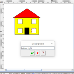 Within FlowframTk, it’s possible to assign descriptions and tags to objects to make them easier to select and find in a complicated image. This post provides an example.
Previous Post

Recent Posts
Within FlowframTk, it’s possible to assign descriptions and tags to objects to make them easier to select and find in a complicated image. This post provides an example. The evolution of a vector graphics application inspired by Acorn's !Draw application designed for integration with LaTeX documents, either exporting images as pgf code or exporting document classes or packages that use the flowfram package. The application was originally named JpgfDraw but was then renamed FlowframTk.There are a growing number of digital historians who are interested in documenting old computing systems from the twentieth century, but much of the information has been lost and coincident names can make it hard to search. This article is about the RISC OS ARMTeX distribution, which provided TeX and LaTeX for the ARM-powered Acorn computers in the 1990s.
 The DRM-free ebook retailer SmashWords has its annual Summer/Winter sale from 1st – 31st July 2025. My crime novel “The Private Enemy” and children’s illustrated story “The Foolish Hedgehog” both have a 50% discount, and my crime fiction short stories “I’ve Heard the Mermaid Sing”, “Unsocial Media”, “Smile for the Camera”, and “The Briefcase” have a 100% discount (i.e. free!) for the duration of the sale. Did you know that you can gift ebooks on SmashWords?
 If you have read my short story Smile for the Camera, did you notice that the ending could have two possible interpretations? (No spoilers please!) As a writer, it’s always difficult to tell if something is too obvious or too obscure. If you need a hint, consider the naming scheme and remember that not everyone is what they say or imply that they are.
Search Blog
📂 Categories
- Autism
- Books
- Children’s Illustrated Fiction
- Illustrated fiction for young children: The Foolish Hedgehog and Quack, Quack, Quack. Give My Hat Back!
- Creative Writing
- The art of writing fiction, inspiration and themes.
- Crime Fiction
- The crime fiction category covers the crime novels The Private Enemy and The Fourth Protectorate and also the crime short stories I’ve Heard the Mermaid Sing and I’ve Heard the Mermaid Sing.
- Fiction
- Fiction books and other stories.
- Language
- Natural languages including regional dialects.
- (La)TeX
- The TeX typesetting system in general or the LaTeX format in particular.
- Music
- Norfolk
- This category is about the county of Norfolk in East Anglia (the eastern bulgy bit of England). It’s where The Private Enemy is set and is also where the author lives.
- RISC OS
- An operating system created by Acorn Computers in the late 1980s and 1990s.
- Security
- Site
- Information about the Dickimaw Books site.
- Software
- Open source software written by Nicola Talbot, which usually has some connection to (La)TeX.
- Speculative Fiction
- The speculative fiction category includes the novel The Private Enemy (set in the future), the alternative history novel The Fourth Protectorate, and the fantasy novel Muirgealia.
🔖 Tags
- Account
- Alternative History
- Sub-genre of speculative fiction, alternative history is “what if?” fiction.
- book samples
- Bots
- Conservation of Detail
- A part of the creative writing process, conservation of detail essentially means that only significant information should be added to a work of fiction.
- Cookies
- Information about the site cookies.
- Dialect
- Regional dialects, in particular the Norfolk dialect.
- Docker
- Education
- The education system.
- Ex-Cathedra
- A Norfolk-based writing group.
- Fantasy
- Sub-genre of speculative fiction involving magical elements.
- File formats
- FlowframTk
- A vector graphics application written in Java that can export to pgf picture drawing code but can also be used to construct frames for use with the flowfram package. Home page: dickimaw-books.com/software/flowframtk. (FlowframTk was originally called JpgfDraw.)
- Hippochette
- A pochette (pocket violin) with a hippo headpiece.
- History
- I’ve Heard the Mermaid Sing
- A crime fiction short story (available as an ebook) set in the late 1920s on the RMS Aquitania. See the story’s main page for further details.
- Inspirations
- The little things that inspired the author’s stories.
- Linux
- Migration
- Posts about the website migration.
- Muirgealia
- A fantasy novel. See the book’s main page for further details.
- News
- Notifications
- Online Store
- Posts about the Dickimaw Books store.
- Quack, Quack, Quack. Give My Hat Back!
- Information about the illustrated children’s book. See the book’s main page for further details.
- Re-published
- Articles that were previously published elsewhere and reproduced on this blog in order to collect them all together in one place.
- Sale
- Posts about sales that are running or are pending at the time of the post.
- Site settings
- Information about the site settings.
- Smile for the Camera
- A cybercrime short story about CCTV operator monitoring a store’s self-service tills who sees too much information.
- Story creation
- The process of creating stories.
- TeX Live
- The Briefcase
- A crime fiction short story (available as an ebook). See the story’s main page for further details.
- The Foolish Hedgehog
- Information about the illustrated children’s book. See the book’s main page for further details.
- The Fourth Protectorate
- Alternative history novel set in 1980s/90s London. See the book’s main page for further details.
- The Private Enemy
- A crime/speculative fiction novel set in a future Norfolk run by gangsters. See the book’s main page for further details.
- Unsocial Media
- A cybercrime fiction short story (available as an ebook). See the story’s main page for further details.
- World Book Day
- World Book Day (UK and Ireland) is an annual charity event held in the United Kingdom and the Republic of Ireland on the first Thursday in March. It’s a local version of the global UNESCO World Book Day.
- World Homeless Day
- World Homeless Day is marked every year on 10 October to draw attention to the needs of people experiencing homelessness.